We need people sounding alarms, because being aware of what could go wrong is how we stop it happening. The warnings that do the most good share two things: they say how the disaster would happen, and they say what could be done about it. That gives people something to act on, and when they act, the warning often ends up looking wrong.

Economic historians, researchers who study emergency warnings, forecasters and AI safety researchers have each worked out a piece of it. So, like in most of my writing, I attempt here to synthesise those thoughts.

The Malthusian trap

In 1798 Thomas Malthus published An Essay on the Principle of Population. His argument was that population multiplies (growing exponentially) while food supply only grows by adding a bit each year (linear growth), so people always end up outnumbering the food until famine, disease or war brings the numbers back down. Judged against the history he had to go on, that was a reasonable reading.

What he didn’t allow for was technology changing how fast food production could grow. He treated the limit as fixed, which, with the benefit of hindsight, we know it wasn’t. So, in assessing any doomsday forecast, the lesson learned is to ask whether it takes today’s limits and projects them forward as though nobody will respond to them.

A warning rather than a prophecy

A hundred years after Malthus, the chemist William Crookes used a major scientific address in 1898 to warn that England and “all civilised nations stand in deadly peril of not having enough to eat.” Wheat needs nitrogen, the Chilean mineral deposits used as fertiliser were running out, and on his figures wheat would fall behind population after 1931. He also said what would fix it: “The fixation of atmospheric nitrogen therefore is one of the great discoveries awaiting the ingenuity of chemists” (The Wheat Problem, the book version of the address). In other words, find a way to turn the nitrogen in the air into fertiliser.

That’s what happened. By 1913 the German chemical company BASF was running Fritz Haber and Carl Bosch’s process for doing exactly that at industrial scale. Though, I can’t say with certainty that Crookes’s speech prompted their work. Haber’s Nobel lecture describes the same worry about the Chilean deposits becoming “clearly apparent at the turn of the century”, without naming Crookes. Either way, Crookes named the fix that came.

Jason Crawford tells this story in Solutionism. He points out that the 1931 shortfall was avoided mostly by things Crookes didn’t foresee: tractors made it pay to farm more land, and new wheat varieties helped. He then sets Crookes against Paul Ehrlich’s 1968 bestseller The Population Bomb. In the passages Crawford quotes, the book opens by declaring “the battle to feed all of humanity is over” and later endorses forcing population control on people: “Coercion? Perhaps, but coercion in a good cause.” Crawford’s distinction is that Crookes’s alarm was contingent, meaning it depended on facts that could change, so “when the facts changed, the alarm could end”. Ehrlich’s, in Crawford’s reading, was “impervious to facts”. Crookes described his own speech, in Crawford’s quotation of him, as taking “the form of a warning rather than of a prophecy”: a warning comes with a way to stop it coming true.

What the research says about warnings

Researchers who study emergency warnings for floods, storms and evacuations reached a similar conclusion from a different direction. A 2018 National Academies review of that work says warnings are more likely to get people to act if they cover “guidance, time, location, hazard and consequences, and source”, and that “people increase responsiveness when they receive guidance on exactly what to do.”

Health researchers have studied fear directly. Scaring people does work, if modestly: a 2015 review of 127 studies found fear-based messages generally changed attitudes and behaviour, and found no case where they backfired. But they worked better when they told people what they could do. An earlier review found that strong fear plus a clear, workable action produced the most change, while strong fear with no workable action produced the most defensive reactions, such as avoiding the message altogether.

On that evidence, a vague warning does less than it could.

From forecasting, the political scientist Philip Tetlock spent years scoring expert predictions, and found that pundits protect themselves “by relying on vague verbiage. They can often be wrong, but never in error.” A warning that never says what would happen, or when, can’t be checked, so nobody can learn from it.

Wrong because they were heeded

The ozone layer is the clearest case of a specific warning working. In 1974 the chemists Mario Molina and Sherwood Rowland showed that CFCs, gases then used in aerosol cans and fridges, could destroy the ozone that shields the Earth from ultraviolet light. That named a mechanism and a fix: stop using CFCs. The warning didn’t act alone. The ozone hole over Antarctica, damage people could actually see, was reported in 1985, two years before the Montreal Protocol to phase the gases out was signed. The UN’s 2023 assessment says the ozone layer is on track to recover within decades.

Looking back, it’s easy to see that as a scare that came to nothing, when the warning did its job. The sociologist Robert Merton had a name for this in 1936, the “suicidal prophecy”, now usually called a self-defeating prophecy: a prediction that changes behaviour enough to make itself untrue.

That’s why “doom predictions have always been wrong” is a weak argument. Some were wrong because the danger wasn’t real and some because the warning worked, and the record doesn’t say which is which. Even the famous bet between Ehrlich and the economist Julian Simon over whether resource prices would rise, which Ehrlich lost, proves less than it seems: Our World in Data found that over other decades since 1900 each man would have won about half the time.

Two kinds of AI warning

It’s easy to assume most AI doom names no mechanism at all. These are the clickbait headlines most of us come across each day. That turns out to be unfair to the researchers. AI safety has its own push for concreteness, going back at least to a 2016 paper literally titled Concrete Problems in AI Safety. A 2023 overview sorts catastrophic AI risk into four groups: people deliberately misusing AI, companies and countries racing to deploy it before it’s safe, accidents inside the organisations building it, and AI systems that can’t be controlled. For each it describes specific hazards and proposes practical fixes.

What reaches most people is a different register. A widely reported statement on AI risk, signed in 2023 by Geoffrey Hinton, Yoshua Bengio and the heads of OpenAI and Google DeepMind among many others, is one sentence long: “Mitigating the risk of extinction from AI should be a global priority alongside other societal-scale risks such as pandemics and nuclear war.” It names no mechanism and no action, and it’s the version I see in the headlines far more often than anything from the papers.

The best case I found for staying vague comes from Eliezer Yudkowsky, one of the most prominent voices on AI risk. In a 2023 piece for TIME he compares humanity facing a superhuman AI to “a 10-year-old trying to play chess against Stockfish 15”, a chess program far stronger than any human. You can be sure you’ll lose without being able to say which moves will beat you, and knocking down one predicted path to disaster wouldn’t make the danger go away. That’s a fair point. His proposed actions are anything but vague, though: “Shut down all the large GPU clusters.” When you can’t predict the path, the only lever left is whether to start the game at all.

Specificity has a trap of its own as well. Amos Tversky and Daniel Kahneman showed in 1983 that adding detail to a scenario makes it feel more likely even as it becomes less likely, because every extra detail is one more thing that has to come true. A vivid story of exactly how AI goes wrong is more persuasive and less probable than a general one. So specificity says nothing about whether a warning is right. What it adds is that the warning can be checked and acted on.

A smaller example of the useful kind: “AI agents that act on content they read can be steered by instructions hidden in that content.” Left alone, that leads to AI assistants leaking data and following attackers’ orders. It names the mechanism, and people are building defences against it right now. If those defences work, the warning will look wrong in a few years, just as Crookes’s does.

Keynes, read properly

See, I’ve come back to Keynes. The passage in A Tract on Monetary Reform (1923) reads “But this long run is a misleading guide to current affairs. In the long run we are all dead.” He was writing about economists who said the quantity theory of money (the idea that prices rise in step with the amount of money in circulation) would hold in the long run, and left it there. His target was people using the long run to shrug off present problems. A doomsayer makes the opposite claim: that the long run is catastrophic. The first half of his quote applies to both, though. A long-run forecast, optimistic or apocalyptic, is a poor guide to what to do now.

A warning worth having about AI

Writing Running to Stand Still left me with one I’d put forward. AI is adding code faster than our ways of checking it have adapted, the code that gets through unchecked carries failures and security holes, and the way out is to make checking much cheaper or to need less code.

The evidence for the first part is real, if indirect. At Google, executives say the share of new code written by AI went from “more than a quarter” in October 2024 to about half by early 2026, with engineers reviewing it. Google’s own DevOps research team found in its 2025 survey of technology professionals that AI adoption goes with less stable software releases, and put that down to checking: without strong automated testing and fast feedback, “an increase in change volume leads to instability.” A study of open-source projects that adopted the AI coding tool Cursor found a large but short-lived jump in how fast they worked, a lasting rise in code-quality warnings, and named “quality assurance as a major bottleneck.” On the second part, a Stanford user study found that people with an AI assistant wrote less secure code than people without one, and were more likely to believe their code was secure.

The same DevOps research also points the other way. Its 2024 report estimated that as AI adoption rose, code reviews got a few per cent faster and code quality a few per cent better, even while releases got less stable. By 2025, AI adoption also went with teams delivering software faster, which the researchers read as people “learning where, when, and how AI is most useful.” Only the link to less stable releases held. So the evidence shows checking under strain, and some sign of it catching up. It doesn’t show checking falling further behind.

Left alone, unchecked code piles up, and so do the failures and security holes hiding in it. That’s a Malthusian trap, with writing code in the role of population and checking it in the role of food.

Malthus missed two things, and each has a counterpart here. The first was a jump in how fast the limited resource could grow: fertiliser changed food production. For code, the equivalent would be checking getting much cheaper, most plausibly through machines writing mathematical proofs that their code is correct, which a small, simple program can then confirm. The second was demand: once people got richer they chose to have fewer children, which Malthus never expected. For code, the equivalent is needing less of it, where more requests get answered with a finished result rather than a program somebody has to trust.

By this post’s own test, the warning falls short of Crookes’s in one way: it has no date. The evidence shows the strain already appearing, and says nothing about when, or whether, it turns into a crisis. I can’t tell you which way out will come either, or whether it’ll be something that isn’t on anyone’s list yet, just as Malthus had no way to foresee synthetic fertiliser.

I’ve concluded not, but for a reason other than I initially expected. Code can get very close to perfect, as long as perfect means doing exactly what it was meant to do at the time it was written. Updates still won’t be features only, because some changes you choose and others the world forces on you. What AI may change is who handles the forced ones. They could turn into something closer to an immune response, happening in the background without anyone deciding on it.

Most of the ideas here come from people who work much closer to these fields than I do, and I’ve credited them as they come up. What I’ve tried to do is put them together in a way that’s digestible for a broad audience, who, like me, are interested but not experts.

Perfect against what

Code can only be correct against something: a specification (spec), which is a precise description of what it should do. Proving code correct against its spec is already possible for some software. seL4, the core of an operating system, and CompCert, a compiler (the program that turns the code people write into instructions a computer runs), both come with mathematical proofs that the code does what its spec says. When researchers fed randomly generated programs to a range of C compilers to hunt for bugs, CompCert was the only one where they couldn’t make the proven part produce wrong results. The bugs they did find were in a part the proof didn’t cover, and in a corner the spec didn’t describe fully.

Those proofs hold under stated assumptions, though. The seL4 team lists theirs: the compiler used to build it, the start-up code and the hardware itself are among the things assumed to work correctly. And the spec has to say what you actually wanted. So a proof moves the question to the spec.

It’s tempting to think that’s where perfect code breaks down, because specs come from people and people get things wrong. Say I build an app to sell hotdogs and it sells hotdogs. Later I realise I should have been selling burgers. Nothing was wrong with the hotdog app. I changed my mind, and the burger version is a new release with that burger-selling feature.

What does count against the code is intent I had at the time and never wrote down. If the hotdog app lets someone order minus three hotdogs and collect a refund, I didn’t change my mind about that. I never wanted it, and the spec never said so. A lot of security vulnerabilities look like this: specs describe what should happen, and rarely list everything that must not.

Machines can close most of that gap, because most unstated intent is shared: no negative quantities, no charging twice, no showing one customer another’s orders. In my experience AI models are good at inferring those, and at finding the gaps and contradictions in a spec. It’s why I now write a scope file before starting a project (see How Long Is a Piece of String?). With a machine checking the spec and a proof tying the code to it, code that is correct against what you intended at the time looks achievable. It rests on proof tools getting much cheaper, which I think we can foresee happening over the coming years.

Decided or imposed

Even if you grant all of that, updates don’t become features only. MD5 and SHA-1 are hash algorithms, used to check that files and digital signatures haven’t been tampered with. A perfectly correct implementation of either is still insecure today, because both were broken after they shipped: MD5 in 2004 and SHA-1 in 2017. RSA, the encryption behind much of the internet’s security, is expected to follow once quantum computers get large enough, which is why the US standards body NIST has already published replacement standards. None of that code had a bug. The world it runs in changed.

You could argue that “I now want to be safe from the new attack” is just another change of intent, which would make it a feature too. Push that far, though, and every change is a feature, so perfect code is perfect by definition and the question stops meaning anything. Perhaps a more useful framing of change:

• Decided: I chose to change it. Burgers instead of hotdogs.
• Imposed: the change is forced on me, and I’d lose something by not making it. An algorithm gets broken, someone else’s code that mine relies on gets withdrawn, a regulator changes the rules.

This framing is at least fifty years old. E. Burton Swanson split software maintenance in 1976 into corrective work (fixing faults), adaptive work (keeping up with a changing environment) and perfective work (improvements people ask for). He described failures and environmental change as causes where “a response is typically unavoidable”, against changes that reflect “the initiatives of user and maintenance personnel”. Manny Lehman’s first law of software evolution says much the same: a program used in the real world “undergoes continual change or becomes progressively less useful.”

What perfect code does to Swanson’s categories is take corrective work, fixing bugs, to near zero. It does nothing about adaptive work, which arrives at the speed the world moves, however good the code is.

Adapt or perish

Put that way, software starts to look like biology. The environment changes and an organism adapts or dies out. Treating software as an evolving ecosystem has a research literature of its own, and a recent example asks what AI coding tools will do to it. Security is a close match for what biologists call the Red Queen hypothesis, after the character in Through the Looking-Glass who has to keep running to stay in the same place. Attackers and defenders evolve against each other, and patching is the running. I’m not the first to make that comparison either.

Biology has no perfect organism, only organisms well suited to the environment they’re in right now. Perfect code works the same way. It can be perfect against its spec at a point in time, and it stops being perfect when the world moves.

The analogy breaks on intent. Evolution has none: variation is random and selection does the work. Software has my “decided” changes too, and they get written straight into the next version. That makes software closer to Lamarck, who thought creatures passed on traits they acquired during their lives, than to Darwin.

An immune system for code

Until now, both kinds of change went through a person. Someone decided on the burgers, and someone noticed the broken hash algorithm and wrote the patch. With AI writing the code, the imposed changes don’t need a person any more. A security hole is announced, the affected code gets updated, the automated tests pass and the fix ships. That works more like an immune system than evolution - your body fights off a cold without you deciding to.

Stephanie Forrest and colleagues were building security on immune-system principles in the 1990s (Computer Immunology, 1997), and software that repairs bugs by itself has been a research field for over fifteen years. It now runs end to end without a person. In DARPA’s AI Cyber Challenge, which finished in August 2025, the finalists’ autonomous systems between them found 18 real vulnerabilities in open-source software and supplied patches for 11.

So from a person’s point of view, updates may well become features only. The imposed changes still happen, but as background maintenance nobody decides on or sees.

When the immune system is the target

An immune system that runs on its own, while convenient, comes with its own perils and becomes a surface worth attacking. Whatever comes in through the update pipeline gets trusted and spread everywhere, so that’s where an attacker should aim. The xz utils backdoor, found in 2024, was an early example: a contributor spent over two years earning the trust of the people who maintain xz, a compression tool built into many Linux systems, then slipped a backdoor in through its normal release process. Automated repair has its own version. A 2025 study wrote 51 fake bug reports aimed at an AI repair system, and 90% of them got it to produce the patch the attacker wanted. In biology the equivalent is a pathogen that exploits the immune response, or an autoimmune disease where the defences attack the body.

The automation also speeds up the environment it’s responding to. When each system adapts on its own, its changes become imposed changes for everything that depends on it, and those systems adapt in turn. The faster systems adapt, the faster the environment around them changes.

Having the same models write the spec, the code and the review makes this worse. As I found with AI code reviews, each run is one sample, and different runs share blind spots, so a miss in the spec can pass straight through all three. In Musings on the Future of Programming Languages I wondered whether reading code might become like reading the raw instructions a processor runs: possible, but rarely needed. If that happens, no person reads the code at all.

Computer scientists proposed a defence for this decades ago. In proof-carrying code, described by George Necula in 1997, code from an untrusted source arrives with a mathematical proof that it follows an agreed set of safety rules, and the system receiving it checks the proof before running anything. Applied here, a model would produce the spec, the code and a proof that one matches the other, and a small, deliberately simple program called a proof checker would confirm the proof is valid. Trust would then rest on the proof checker, which is small enough for people to audit. It only protects what the spec describes, though. A tampered spec gets through, and so does an attack like the xz backdoor, which was hidden in the build process rather than in the code a proof would cover.

So code can get close to perfect and still need patching for as long as the world keeps changing. If machines take that patching over, the immune system becomes the thing to protect. Proof checking is one way to protect it, and it can only be as good as the spec.

Send the source

• Send the Markdown, or whatever the page was rendered from. A person can read it as it is and render it if they want. It was the cheapest copy for Claude to read, and it’s the only one with no rendering step to lose anything in.
• Don’t send a link to a web page. In my tests the agent got only a short summary of the page, and once said it had read the whole thing.
• If Claude published the document as an artifact, ask it for the Markdown too and send that.
• Don’t send a single-file Quarto page. With only its Read tool, Claude couldn’t read it at all.
• Don’t rely on a PDF. Most of the tools that make one can break file paths across lines, and Claude doesn’t always put them back together. If you do print one from a browser, set inline code to white-space: nowrap first.

A link

A pasted link to an ordinary web page goes through WebFetch, which by Claude Code’s own description converts the page to Markdown and has “a small fast model” answer a prompt about it. The agent gets that answer. I gave a session the arXiv link for Attention Is All You Need and asked it to read the whole page. It got back two short answers from a 189 KB page and replied that it had read it. In a second session on a newer Claude Code, it got the same kind of answers and said it couldn’t honestly claim to have read the page.

Claude can also publish a document as an artifact, a page on claude.ai you share by link. My review of my tidylearn package went out that way, with no Markdown copy. I tried the ways an agent could read it. Each copy was read in full, one session per copy, and the tokens each read added come from the session’s own usage records.

WebFetch didn’t get the page in any session I measured. Told to use it, it got HTTP 403 each time. Left to choose, the agent didn’t try, saying it couldn’t open claude.ai links, and asked for the content to be pasted in. Those were headless sessions (claude -p). In my own interactive session in VS Code, WebFetch opened the same link through my claude.ai login and returned it the way the Artifact tool does. So what WebFetch gets depends on the session, and I haven’t pinned down which part of it matters.

The tidylearn page is over 50 KB. The Artifact tool handed over the first 50 KB and saved the whole file to disk with an instruction to read all of it. In two sessions the agent then read the whole file, so most of the page went in twice. In a third, on a newer Claude Code, it read only the part it hadn’t seen. Two smaller artifacts of mine came back whole in one call. Having the Artifact tools available also adds context to every call a session makes, whether or not it reads an artifact.

I own this artifact, which is why the tool gave me its HTML. For an artifact someone else shared with you, the tool’s own description says a read returns an isolated summary. That’s the usual case for the engineer, and a summary can drop exactly the file paths and line numbers the engineer’s session needs.

Turning the page into Markdown after the fact was harder than it should be. The content isn’t in the HTML as text: a script builds it in the browser, so pandoc turned the saved page into an empty file. I had to render the page in a headless browser first. Asking Claude for the Markdown when it writes the document avoids all of that.

Rendered copies

The other document is a review Claude wrote for a new product feature: 12 KB of Markdown with headings, lists, and file paths and line numbers in code formatting. I rendered it to HTML with pandoc, to a single-file HTML page with Quarto (embed-resources, which is what makes it one file you can send), and to PDF by printing the pandoc page from Chrome. Claude read each copy with its Read tool.

With only its Read tool, Claude never got through the Quarto page. Quarto packs the page’s scripts, fonts and stylesheet into the file, some of them as single lines too long for the Read tool to return, and the report itself starts more than two thousand lines in. Claude hit one of those lines, couldn’t get past it, and said it could not read the file. Given search tools as well, it found where the report starts and read it from there, adding about three times the tokens the Markdown did.

The PDF broke file paths. Pandoc’s stylesheet lets inline code wrap, and Chrome treats a hyphen as a place to break a line, so a path like load-model.ts:120-135 can end up split across two lines. Word and LibreOffice do the same. Typst breaks paths at slashes too, and LaTeX keeps them whole but lets a long one run off the edge of the page. Pull the text back out of a split path and you get a line break in the middle of it, or the hyphen gone: loadmodel.ts. The HTML kept every path exactly as written.

Claude usually put split paths back together, but not always. On two synthetic reviews with known paths, it gave every split path back exactly on one, and on the other some reads came back with a hyphen missing: statement-run-8 as statement-run8. Adding code { white-space: nowrap; } to the page before printing from Chrome stopped the splits: each path moved whole to the next line.

What it costs

For a light document the difference is small. The Markdown session above cost $0.070 at list price and the PDF session $0.101, against $0.046 for a session with no document. The PDF cost the most because a short PDF goes in as a document block, which Anthropic’s documentation says carries each page as an image with its extracted text alongside, so Claude got it twice.

The dollar figures are Claude Code’s list prices, which is the unit it reports. On a subscription you won’t see a bill for any of this: the figures are a weighting for how much of your usage limit each copy takes up.

Whatever a read adds stays in the session, and every later call sends it again, from the prompt cache, until you /clear. Cache reads are billed at a fraction of normal input, so for a light document that stays small.

Heavy markup costs far more. The arXiv HTML page of Attention Is All You Need added 101.8K tokens against 19.4K for its PDF, and that session cost $0.59 at list price against $0.13.

What the numbers do not cover

• A link someone else shared with you. The artifact was read by the account that owns it, and the shared case, where the agent gets a summary, isn’t measured.
• Your own documents. A page with heavier markup than my reports will cost more to read, and a different renderer may break different things. The scripts in the footer run the same checks on your files.
• Other models. Everything ran on Sonnet 5 at low effort, and another model or effort level may repair broken paths more or less reliably.
• Other web pages. WebFetch was tried on one page, and another may come back differently.
• The measured sessions were headless. An interactive session can behave differently, as WebFetch did with the artifact link.
• The path checks show whether exact paths survive. They don’t show whether Claude understood the rest of a document.

The rendered report and the paper were recorded on 16 September 2026 and everything else on 17 September, all on Claude Sonnet 5 at low effort, on Claude Code 2.1.272 except the link sessions repeated on 2.1.273. The WebFetch 403s, a second 2.1.272 Artifact-tool read of the tidylearn page (46.4K) and the interactive WebFetch call come from sessions that aren’t saved. The scripts and the saved runs are in the tokenwise repository, under experiments/doc-format, whose README has the figures left out here and the command to reprint each table for free. The report is a client document and isn’t published, and the artifacts are private, so their saved runs record hashes and versions but not the documents or links. measure.mjs measures your own files and links, pdf-wrap.mjs checks which paths survive each PDF tool without spending anything, and recall.mjs checks whether Claude gives the paths back. The 94 sessions behind the saved runs came to $9.96 at list price.

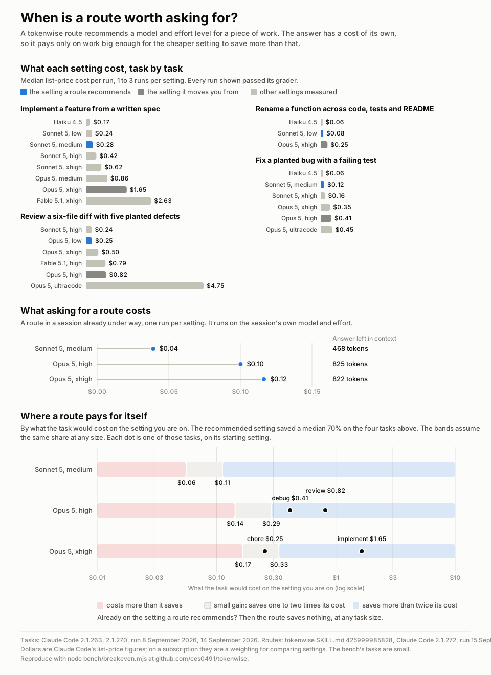
I measured the cost of asking from three session settings and set it against what the cheaper settings saved on the benchmark behind the plugin’s routing table.

What asking costs

A route runs on whatever model and effort your session is on, in a forked subagent, so only its answer comes back into the conversation.

Claude Code’s model configuration docs put Max, Team Premium, Enterprise and API users on Opus 5 at high effort unless they change it, so the middle row is the default on those plans.

That context is carried on every later call until you clear. Anthropic’s pricing page lists an Opus 5 cache read at $0.50 per million tokens, so 825 tokens comes to $0.0004 a call.

Each session routed the same two short task descriptions. Sonnet 5 at medium recommended the same settings for both as the Opus sessions did, at less than half their cost. Its answers ran to 173 and 175 words against 308 to 371 for Opus.

What a cheaper setting saves

Four of the benchmark’s tasks, all against a small invoicing library, ran on the expensive setting a routing claim was tested against and on the setting a route recommends. Every run in these cells passed its grader.

The median saving across the four is 70%.

Where the line falls

A route is told to read only its own instructions and the one-line description you give it, so the size of the work should not change its cost, though the benchmark only priced it on short descriptions. What it saves grows with the work. With a 70% saving, a route breaks even on a task whose cost on your current setting is the route’s cost divided by 0.7, and it saves more than twice its cost only on tasks twice that size.

The bands are worked from the unrounded route costs, so dividing the rounded ones above can land a cent out.

The rename lands in the middle band. It cost $0.25 on Opus at xhigh, moving it to Sonnet at low saved $0.17, and asking cost $0.12, so asking came out $0.05 ahead. That is a gain too small to be worth the typing. The feature, the bug fix and the review each landed where a route saves more than twice its cost.

A route saves nothing when the session is already on the setting it recommends, and then its whole cost is lost whatever the size of the task.

In practice that comes down to three habits:

• For a quick edit, pick a setting yourself: Sonnet at low effort, or Haiku.
• For a feature, a debugging session or a review, ask at the start of the phase, then /clear before you switch, so the switch does not re-process the conversation on the new setting. Switch with s in the /model picker: typing /model <name> also saves it as your default for new sessions.
• When you already know which setting the work needs, skip the question.

What the numbers do not cover

The benchmark’s tasks are small, and every saving above was measured at that size. The bands assume a larger task saves the same share on the cheaper setting, which is untested. If the cheaper setting fails and you run the task again, the retry comes off the saving.

The dollar figures are Claude Code’s list prices. On a subscription they are a weighting for comparing settings.

Changing model on a conversation already under way re-processes all of it on the new model, and so does changing effort on most models, according to Claude Code’s prompt caching docs. Straight after a /clear, only the system prompt and project context are re-processed, as in a new session. A switch without one adds a cost these figures leave out.

The route costs come from one run per setting. The 1.1.1 route, run twice on identical text, cost $0.155 and $0.129, so two runs of one route can differ by $0.025, against the rename’s $0.05 margin. Sonnet 5 at high, the default on Pro and Team Standard plans, was not measured.

Task runs on Claude Code 2.1.263, 8 September 2026. Routes on tokenwise 1.3.0 and Claude Code 2.1.272. The code, the transcripts and the chart’s generator are at github.com/ces0491/tokenwise, and two commands check the figures without spending anything: node bench/breakeven.mjs --check confirms the chart follows from the committed runs, and node bench/skill-cost.mjs --compare 1.3.0,1.3.0-opus-high@1.3.0,1.3.0-sonnet-medium@1.3.0 prints the route costs from the saved sessions.

Every API call re-sends the whole conversation. What a task consumes is context size multiplied by the number of calls, and the model and effort level you pick set the rate on top of that.

On my own Claude Code transcripts the input side runs 444 tokens for every one of output, and almost all of it is conversation being re-read from cache. node bench/context-profile.mjs in the repository below produces that table from your transcripts instead of mine.

That leaves two levers. Context size is mostly a discipline problem: when you clear, what you delegate to a subagent, how large a slice you take on at once. tokenwise is for the other one, the model and effort you pick — a decision made once at the start and then usually left alone for the rest of the session.

What it does

Its core is one skill:

/tokenwise:route implement the plan in docs/plan.md, about 12 files

The answer names a model and an effort level and how to switch to them for the session, says whether to clear the context first and what the switch costs if you don’t, says what to push into subagents, says what the cheaper choice gives up, and gives you one check to run to know the phase is finished before you trust it.

Every row of the routing table underneath it names where to start, and the seven rows with somewhere to escalate to name what has to go wrong before you move. The escalation rule comes from Anthropic’s own guidance: if the model failed with the context it had, it did not know enough, so change the model; if it skipped files or stopped early, it did not try hard enough, so raise the effort. I used to treat those as one problem.

Reviewing a diff starts on the expensive model at low effort. High effort on a diff you can hold in your head buys more turns spent re-reading it, and the bound on what a review can usefully do is the subject of How Long Is a Piece of String?.

A second skill, /tokenwise:setup, makes Sonnet 5 at medium the default for new sessions if you say yes. Two hooks warn when resuming a conversation or switching model is about to re-send it to an empty cache, and write nothing into the conversation.

What it will not do

It cannot switch anything for you. Nothing can change a running session’s model or effort level — that is /model and /effort, typed by you. The skill recommends, and tells you what the recommendation gives up.

What the plugin does add to every session is the route skill’s description, 153 tokens, so that Claude knows the skill is there. That also means Claude can run the skill without being told to, and in testing it did when a session asked in plain words which model and effort to use.

What it does not know

Five of the nine rows in the routing table carry no measurement behind them, and each says so in the table. They are informed guesses about work I have not benchmarked.

The four that are measured come from a benchmark I built to check the table, and it changed the table. Four of the eight claims I had written in turned out to be wrong: twice by recommending a setting more expensive than the work needed, once by overstating a saving, and once on a piece of process that charges you for writing a plan down and reading it back. That is its own story and I have written it up separately.

The benchmark counts in dollars, because list prices are the unit Claude Code reports. On a subscription they measure how much of your month a task eats rather than a charge you will see.

Every graded run passed, whatever the setting, so the benchmark compares consumption at equal outcomes and never reaches the point where an expensive setting earns its keep by succeeding where a cheap one fails. The graders, the pre-registered pass criteria and the raw results for every run are in the repository, so you can disagree with me using my own data.

Install

/plugin marketplace add ces0491/tokenwise
/plugin install tokenwise@ces0491-plugins

Or read it before you install it:

git clone https://github.com/ces0491/tokenwise && cd tokenwise
node bench/summarize.mjs --check    # do the published tables follow from the published runs?
node bench/context-profile.mjs      # the token figures above, against your own transcripts

Neither makes an API call, so your limit is untouched. MIT licensed, at github.com/ces0491/tokenwise.

What sent me back to it was a different bug. The momentum factor had been dividing a package’s lifetime downloads by twelve months whether or not it had been on CRAN that long, so a package four months old got a baseline three times too low and its decline came out as growth. Pulling on that thread began to expose a few other gaps.

So: 600 packages spaced evenly through the 24,887 CRAN publishes, in name order, and cranlogs for last month’s totals in three batched requests.

idx  <- available.packages(repos = "https://cloud.r-project.org",
                           filters = character())
pkgs <- sort(rownames(idx))
sel  <- unique(pkgs[round(seq(1, length(pkgs), length.out = 600))])

counts <- unlist(lapply(split(sel, ceiling(seq_along(sel) / 200)), function(ch) {
  jsonlite::fromJSON(paste0(
    "https://cranlogs.r-pkg.org/downloads/total/last-month/",
    paste(ch, collapse = ",")))$downloads
}), use.names = FALSE)

median(counts)
#> [1] 277.5
sum(counts >= 100 & counts < 1000)
#> [1] 532
min(counts)
#> [1] 100

532 of the 600 in one band. The median package gets 277 downloads a month. The factor was carrying a fifth of the weight and telling me almost nothing: a package on 150 a month sits at the 4th percentile of that sample, one on 900 sits at the 88th, and both scored 6 out of 20.

The part I hadn’t gone looking for was the band underneath. Labelled very low, and empty. The smallest count anywhere in 600 packages was exactly 100.

It turns out that cranlogs counts fetches from Posit’s mirror, and crawlers and mirror syncs get counted alongside installs. The raw logs record the R version a client reported, and a fetch with none didn’t come from install.packages(). I sampled 9 packages over 13 days: the share reporting a version ran from 9% to 54%, lowest for the packages with the fewest downloads. Nothing on CRAN reads as zero, and the smaller the package, the less of its count is people.

Then I went looking for prior art, in the wrong order. Peter Li shipped packageRank in 2019 and wrote the caveat up in 2020, working from the raw logs rather than the aggregates. Had I read that before writing the scoring code, I’d have started from his caveats instead of reconstructing a rougher version of them.

The bands now break at 50, 200, 500, 2,000, 10,000 and 100,000, cut finer through the range the packages are actually in and left as absolute counts: a few hundred downloads a month is a small user base however much of the repository it beats.

The same pass turned up two more. Maturity was using release count as a proxy for age, and the two correlate at 0.49. Having no reverse dependencies was rendering as a red flag, when 17,313 of the 24,887 packages on CRAN have none.

All of it had been live since the end of March, getting the obvious cases right. ggplot2 near the top, an archived package near the bottom, which seemed like common-sense sniff tests. The errors sat in the middle of the distribution, which is the only part anyone really needs a score for. Sometimes a sniff test is good enough — not everything you build needs to be bulletproof — but I’ve been shown time and time again to never stop pulling on the threads.

Figures from a live run on 4 September 2026; cranlogs totals move daily.

The decision to depend on something is made in a moment, usually while you’re focused on something else entirely — you need a date parser, someone on Stack Overflow (remember Stack Overflow?) used this one, it works, move on. But every so often, the package stops building against the current R release, or the maintainer’s email starts bouncing, or CRAN archives it and that glossed-over reverse dependency becomes a proper headache.

We’ve built good habits around a lot of things that are cheaper to get wrong than this. We review pull requests that change five lines but we don’t review the line that adopts twelve thousand lines of somebody else’s code. Which probably says more about human nature than the explicit habits of coders, but I digress.

CRAN already publishes the answer

The information you’d want is public, free, and machine-readable. It’s just spread across three separate services, none of which is the page you land on when you Google a package name.

• crandb has package metadata, the full release timeline, reverse dependency listings (with a caveat I’ll come back to), and — importantly — whether the package has ever been archived.
• cranlogs has download counts, daily or aggregated over arbitrary windows.
• search.r-pkg.org does full-text search across all of it.

Most of us don’t check all three before adding a dependency. At least, I didn’t. I was fortunate enough to have good training that made me think about these sorts of things but the overhead of a thorough package audit was just too boring and honestly a bit hand-wavy — if there was a good enough package to do a job you needed, you used it. But we have AI for these boring jobs now (like writing tests — I’ve never seen this many tests in repos ever [which is great btw]) so there’s no longer an excuse to implement the good practices you know you should be but don’t.

The five signals

Five signals are worth weighing. Each is easy to over-read on its own, which matters more than the list.

Recency. When was the last CRAN release? This is the signal most reach for but is also easy to misinterpret. A package with no release in three years might be abandoned — or it might be finished. Some of the best small packages on CRAN do one thing, do it correctly, and have had no reason to change. Recency only becomes damning in combination: a long gap plus failing checks on current R is a package on its way to the archive. A long gap plus clean checks is often just a stable package.

Download momentum. What matters is the direction. A package whose downloads have halved over a year is telling you something that its lifetime total is hiding. It is the most forward-looking of the five, and the easiest to compute wrong. cranlogs returns rows only from a package’s first publication, so a four-month-old package has four months of data. Divide its total by twelve to get a baseline and you understate that baseline threefold, which turns a decline into growth. Compare mean downloads per day over the last 30 days against the mean per day over the days before them, and report nothing at all with fewer than 60 days of history.

Download volume. Useful, but inflated. cranlogs counts fetches from Posit’s mirror, so it is a sample of CRAN, and crawlers and mirror syncs are counted alongside installs. Installing a package also pulls its dependencies down with it, which means anything sitting in a popular dependency tree posts numbers that reflect its dependents’ popularity and not necessarily its own adoption. Peter Li made that point, and the observation that the bias dilutes as real downloads rise, in packageRank and his write-up of it. A package with two million downloads a month might have very few humans who chose it deliberately.

Ecosystem adoption. How many other CRAN packages depend on this one. It functions as a form of insurance: CRAN is reluctant to archive a package that would break a long tail of dependents, and maintainers of widely-depended-on packages get pressure, help, and sometimes successors in a way that solo packages don’t. High reverse dependency counts mean the ecosystem itself has a stake in the thing continuing to work.

Maturity. How long the package has been on CRAN. This separates something first published in 2007 from something first published six months ago, which the other four signals can’t distinguish. It’s the weakest of the five, and weighted accordingly, but it captures the case where seemingly promising new packages are relegated on the author’s list of priorities.

Using release count as proxy for age proves a poor decision. Across a systematic sample of 140 CRAN packages the two correlate at 0.49, and 17 of them had been on CRAN eight years or more with four releases or fewer — stable packages that a release-count measure files as new. Take the age from the first publication date, and show the release count beside it as a track record.

Doing it yourself

You don’t need an app for this. Two API calls and one base R function get you most of the way:

library(httr2)

# The slow part; available.packages() caches for the session.
cran_db <- available.packages(repos = "https://cloud.r-project.org")

cran_signals <- function(pkg, db = cran_db) {
  meta <- request("https://crandb.r-pkg.org") |>
    req_url_path_append(pkg, "all") |>
    req_perform() |>
    resp_body_json()

  dl <- request("https://cranlogs.r-pkg.org") |>
    req_url_path_append("downloads", "total", "last-month", pkg) |>
    req_perform() |>
    resp_body_json()

  revdeps <- tools::package_dependencies(
    pkg, db = db, reverse = TRUE,
    which = c("Depends", "Imports", "LinkingTo")
  )[[1]]

  dates <- sort(unlist(meta$timeline))

  list(
    version       = meta$latest,
    first_release = unname(as.Date(dates[1])),
    last_release  = unname(as.Date(dates[length(dates)])),
    releases      = length(dates),
    revdeps       = length(revdeps),
    archived      = meta$archived,
    downloads_30d = dl[[1]]$downloads
  )
}

str(cran_signals("ggplot2"))

List of 7
 $ version      : chr "4.0.3"
 $ first_release: Date[1:1], format: "2007-06-01"
 $ last_release : Date[1:1], format: "2026-04-22"
 $ releases     : int 55
 $ revdeps      : int 4833
 $ archived     : logi FALSE
 $ downloads_30d: int 2000824

Nineteen years, 55 releases, two million downloads a month, 4,833 packages depending on it, never archived. You didn’t need the data to know ggplot2 is safe — if your method disagrees with the obvious cases, you probably need to go back and check your working.

The archived field is worth singling out. A package that has been archived and restored has already demonstrated the failure mode you’re worried about, and it’s the one signal here that’s binary rather than a matter of degree.

crandb has two reverse dependency numbers and one of them is a trap

The reverse dependency count above doesn’t come from the same call as everything else - deliberately.

The /{package}/all response carries a revdeps field. It arrives in the JSON you already have, it’s a single integer, and it is very tempting. It also isn’t the number you want:

dplyr and jsonlite both come back with 63, though dplyr has three times as many actual dependents, and httr2 has no value at all. Whatever that field counts, it isn’t what its name suggests, and a score weighted on it would be ranking packages by an artefact.

The number you actually want is at a different crandb endpoint, /-/revdeps/{package}, which returns the dependent package names split by relationship:

revdeps <- request("https://crandb.r-pkg.org") |>
  req_url_path_append("-", "revdeps", "ggplot2") |>
  req_perform() |>
  resp_body_json()

lengths(revdeps$ggplot2)
#>   Imports  Suggests   Depends  Enhances
#>      4440      2033       395         7

That agrees with tools::package_dependencies() to within a handful of packages — 4,835 against 4,833 — and the difference is just which mirror snapshot each one saw. Either route is correct. The single integer in the metadata blob is not.

The discrepancy is only visible if you already have a sense of the right magnitude. When you assemble a metric from convenient sources, the field that’s easiest to reach is not always the field you want, and a plausible wrong number is much harder to notice than a missing one.

The Score

Five signals is four more than most people will weigh in the few seconds the decision actually gets. So I collapsed them into a 0–100 viability score, weighted like this:

Those weights are a judgement call. Recency and momentum are the forward-looking signals and volume is the backward-looking one, so the front of the list gets the weight — but somebody with different priorities should weight them differently.

The score is a triage tool. It’s good for sorting a shortlist and for noticing that something you assumed was fine has been declining. It is not a verdict, and a low score on a small, finished, well-written package that does exactly what you need is probably a false alarm you should overrule.

The app

I built cranExploreR. It’s a Shiny app — bslib, plotly, httr2 — that pulls the signals above, draws the twelve-month download trend, and lets you put two or three candidate packages side by side, which is usually the actual question.

It’s running here. Source code on GitHub.

The app is convenient but the question is answerable from data CRAN has been publishing all along.

The tooling is there too. packageRank has been on CRAN since 2019, across 25 releases, and treats the download half of this more carefully than anything above — it works from the raw logs rather than the aggregates, which is what it takes to separate an install from a crawler. The data and the tools were both available the whole time. But the percieved overhead of maintaining the discipline of checking meant I wasn’t always doing this. I hope that cranExploreR makes the check trivial enough for it to always be a part of any of your consequential workflows.

The Reporting Problem

Machine learning in R is powerful, but reporting the results often takes more effort than building the model itself. Every package returns results in a different format — a named vector here, a matrix there, a custom S3 object somewhere else. Even with excellent tidying packages like broom, the column names and available fields change between model types, and many ML packages aren’t supported at all.

The result is that producing consistent, polished visualisations and tables for a report means writing custom extraction and reshaping code for each package you use. Change your model, and your reporting code breaks.

tidylearn solves this. Every function — across 20 algorithms — returns tidy tibbles, ggplot2 plots, and formatted gt tables with a consistent structure. Your reporting pipeline becomes model-agnostic: swap the algorithm, and the same plot code, table code, and comparison logic work without modification.

This post walks through real-world analysis tasks — PCA, hierarchical clustering, regularisation, and multi-model classification — comparing the tidylearn workflow against the traditional approach.

library(tidylearn)
library(dplyr)
library(ggplot2)
library(gt)
library(tibble)

1. PCA: Biplot, Scree Plot, and Variance Tables

PCA is a staple of exploratory analysis, and producing a polished biplot or scree plot is one of those tasks that should be straightforward but rarely is.

With tidylearn

pca <- tidy_pca(USArrests, scale = TRUE)

Scree plot with cumulative variance line and 80% threshold:

tidy_pca_screeplot(pca)

Publication-ready biplot with observation scores and variable loadings:

tidy_pca_biplot(pca, label_obs = TRUE)

And the tables — variance explained and loadings — are one call each, with colour-coded formatting out of the box:

pca_model <- tl_model(USArrests, method = "pca")
tl_table_variance(pca_model)

tl_table_loadings(pca_model, n_components = 2)

The loadings table uses a diverging red–blue colour scale to highlight strong positive and negative loadings — no manual formatting required.

Without tidylearn

pca_base <- prcomp(USArrests, scale. = TRUE)

The default R biplot:

biplot(pca_base)

This produces a functional but visually rough base R graphic — no theme_minimal(), no consistent colour scheme, no variance-explained axis labels. To get a ggplot2 biplot, you need to manually extract and scale the scores and loadings:

# Extract scores
scores <- as.data.frame(pca_base$x[, 1:2])
scores$label <- rownames(scores)

# Extract loadings and scale to match scores
loadings <- as.data.frame(pca_base$rotation[, 1:2])
loadings$variable <- rownames(loadings)
score_range <- max(abs(scores[, 1:2]))
loading_range <- max(abs(loadings[, 1:2]))
scale_factor <- (score_range / loading_range) * 0.8

loadings$PC1_scaled <- loadings$PC1 * scale_factor
loadings$PC2_scaled <- loadings$PC2 * scale_factor

# Compute variance explained for axis labels
var_exp <- pca_base$sdev^2 / sum(pca_base$sdev^2) * 100

# Build the ggplot manually
ggplot() +
  geom_point(data = scores, aes(x = PC1, y = PC2),
             colour = "steelblue", alpha = 0.7) +
  geom_text(data = scores, aes(x = PC1, y = PC2, label = label),
            size = 2.5, vjust = -0.5) +
  geom_segment(data = loadings,
               aes(x = 0, y = 0, xend = PC1_scaled, yend = PC2_scaled),
               arrow = arrow(length = unit(0.2, "cm")),
               colour = "red", alpha = 0.7) +
  geom_text(data = loadings,
            aes(x = PC1_scaled, y = PC2_scaled, label = variable),
            colour = "red", size = 3, fontface = "bold", vjust = -0.5) +
  labs(
    title = "PCA Biplot",
    x = sprintf("PC1 (%.1f%% variance)", var_exp[1]),
    y = sprintf("PC2 (%.1f%% variance)", var_exp[2])
  ) +
  coord_equal() +
  theme_minimal()

# Variance table — manually computed
var_explained <- data.frame(
  component = paste0("PC", seq_along(pca_base$sdev)),
  sdev = pca_base$sdev,
  variance = pca_base$sdev^2,
  prop_variance = pca_base$sdev^2 / sum(pca_base$sdev^2),
  cum_variance = cumsum(pca_base$sdev^2 / sum(pca_base$sdev^2))
)

knitr::kable(var_explained, digits = 3,
             caption = "Variance Explained (manual)")

Variance Explained (manual)

The manual biplot requires extracting matrices, scaling loadings to match score ranges, computing variance percentages for axis labels, and assembling the ggplot layer by layer. tidy_pca_biplot() handles all of that in one call. And the kable() variance table is functional but plain — no colour coding, no cumulative-variance highlighting. tl_table_variance() adds these by default.

2. Hierarchical Clustering

Hierarchical clustering involves computing distances, fitting the tree, visualising the dendrogram, cutting it, and augmenting your data with cluster assignments. Each step traditionally produces a different data structure.

With tidylearn

hc <- tidy_hclust(USArrests, method = "ward.D2")

# Dendrogram with cluster rectangles
tidy_dendrogram(hc, k = 4)

Cut the tree and get a tidy tibble of cluster assignments:

clusters <- tidy_cutree(hc, k = 4)
knitr::kable(head(clusters, 10), caption = "Cluster Assignments (first 10)")

Cluster Assignments (first 10)

Augment the original data and produce a formatted cluster summary table:

hc_model <- tl_model(USArrests, method = "hclust")
tl_table_clusters(hc_model, k = 4)

Without tidylearn

# Compute distance matrix
d <- dist(scale(USArrests), method = "euclidean")

# Fit hierarchical clustering
hc_base <- hclust(d, method = "ward.D2")

# Plot dendrogram
plot(hc_base, main = "Hierarchical Clustering Dendrogram",
     xlab = "", sub = "", cex = 0.7)
rect.hclust(hc_base, k = 4, border = 2:5)

The dendrogram looks similar — both use base R graphics for this. The real difference is in what happens next:

# cutree returns a named integer vector — not a tibble
clusters_base <- cutree(hc_base, k = 4)
str(clusters_base)
#>  Named int [1:50] 1 2 2 3 2 2 3 3 2 1 ...
#>  - attr(*, "names")= chr [1:50] "Alabama" "Alaska" "Arizona" "Arkansas" ...

# To get a summary table, manually bind and reshape
USArrests_clustered <- USArrests
USArrests_clustered$cluster <- clusters_base

USArrests_clustered %>%
  group_by(cluster) %>%
  summarise(across(where(is.numeric), mean), .groups = "drop") %>%
  knitr::kable(digits = 1, caption = "Cluster Means (manual)")

Cluster Means (manual)

The dendrogram itself is comparable. But cutree() returns a named integer vector that needs manual binding to your data, and the resulting kable() is plain text. tl_table_clusters() produces a formatted table with cluster sizes, styled headers, and consistent theming — ready for a report.

3. Lasso Regularisation: Coefficient Paths and Tables

Regularised models are a common choice, but visualising how coefficients shrink along the regularisation path is one of those tasks where the default output is decidedly not report-ready.

With tidylearn

lasso <- tl_model(mtcars, mpg ~ ., method = "lasso")

# Coefficient path as a ggplot2 object
tl_plot_regularization_path(lasso)

# Cross-validation curve
tl_plot_regularization_cv(lasso)

And a formatted coefficient table, sorted by magnitude with zero coefficients greyed out:

tl_table_coefficients(lasso)

Both plots are ggplot2 objects — theme_minimal(), consistent aesthetics, and directly passable to ggplotly() or ggsave(). The table is a gt object with the same consistent styling.

Without tidylearn

library(glmnet)

# Prepare model matrix (glmnet doesn't accept formulas)
x <- model.matrix(mpg ~ ., data = mtcars)[, -1]
y <- mtcars$mpg

# Fit with cross-validation
cv_fit <- cv.glmnet(x, y, alpha = 1)

The default coefficient path plot:

plot(cv_fit$glmnet.fit, xvar = "lambda", label = TRUE)

The default cross-validation plot:

plot(cv_fit)

These are base R graphics — functional, but they can’t be themed, faceted, combined with other ggplot2 panels, or converted to interactive plotly charts. Building ggplot2 equivalents from the glmnet object requires extracting the coefficient matrix across all lambda values and pivoting it to long format:

# Extract coefficient matrix
coef_matrix <- as.matrix(cv_fit$glmnet.fit$beta)
lambda_vals <- cv_fit$glmnet.fit$lambda

# Reshape to long format for ggplot
coef_df <- as.data.frame(t(coef_matrix))
coef_df$lambda <- lambda_vals
coef_long <- tidyr::pivot_longer(coef_df, -lambda,
                                  names_to = "variable",
                                  values_to = "coefficient")

ggplot(coef_long, aes(x = log(lambda), y = coefficient, colour = variable)) +
  geom_line() +
  labs(title = "Lasso Coefficient Path", x = "log(lambda)",
       y = "Coefficient", colour = "Variable") +
  theme_minimal()

# Extract coefficients at lambda.1se — returns a sparse matrix
coefs <- as.matrix(coef(cv_fit, s = "lambda.1se"))
coef_tbl <- data.frame(
  term = rownames(coefs),
  estimate = as.vector(coefs)
)
coef_tbl <- coef_tbl[order(-abs(coef_tbl$estimate)), ]

knitr::kable(coef_tbl, digits = 4, row.names = FALSE,
             caption = "Lasso Coefficients at lambda.1se (manual)")

Lasso Coefficients at lambda.1se (manual)

The manual approach works, but it’s the kind of reshaping code that’s easy to get subtly wrong and tedious to repeat. tl_plot_regularization_path() handles extraction, pivoting, labelling, and theming in one call. And the kable() coefficient table is plain — tl_table_coefficients() adds sorting, zero greying, and the selected lambda value in the subtitle.

4. Multi-Model Classification Comparison

Comparing models across packages is where consistent output structure matters most. Each package has its own prediction interface, metric accessors, and plot conventions.

With tidylearn

split <- tl_split(iris, prop = 0.7, stratify = "Species", seed = 42)

# Fit three models — same interface for each
m_forest   <- tl_model(split$train, Species ~ ., method = "forest")
m_tree     <- tl_model(split$train, Species ~ ., method = "tree")
m_xgboost  <- tl_model(split$train, Species ~ ., method = "xgboost")

A formatted comparison table — one call:

tl_table_comparison(
  m_forest, m_tree, m_xgboost,
  new_data = split$test,
  names = c("Random Forest", "Decision Tree", "XGBoost")
)

And a confusion matrix for any model:

tl_table_confusion(m_forest, new_data = split$test)

Adding a fourth model is just another argument in tl_table_comparison() — the table code stays unchanged.

Without tidylearn

library(randomForest)
library(xgboost)

set.seed(42)
train_idx <- unlist(lapply(
  split(seq_len(nrow(iris)), iris$Species),
  function(i) sample(i, size = floor(0.7 * length(i)))
))
train_data <- iris[train_idx, ]
test_data  <- iris[-train_idx, ]

# Two of the three take a formula and a data frame
fit_rf   <- randomForest(Species ~ ., data = train_data)
fit_tree <- rpart::rpart(Species ~ ., data = train_data, method = "class")

# xgboost takes neither: a numeric matrix, integer-encoded labels, and
# xgb.train() rather than xgboost(), which refuses multiclass outright
dtrain <- xgb.DMatrix(
  data  = as.matrix(train_data[, 1:4]),
  label = as.integer(train_data$Species) - 1
)
fit_xgb <- xgb.train(
  params  = list(objective = "multi:softmax", num_class = 3),
  data    = dtrain,
  nrounds = 20,
  verbose = 0
)

# Each returns predictions in a different format
pred_rf   <- predict(fit_rf, newdata = test_data)
pred_tree <- predict(fit_tree, newdata = test_data, type = "class")
pred_xgb  <- predict(fit_xgb, xgb.DMatrix(as.matrix(test_data[, 1:4])))

# And the xgboost predictions are zero-based integers, not factor levels
acc_rf   <- mean(pred_rf == test_data$Species)
acc_tree <- mean(pred_tree == test_data$Species)
acc_xgb  <- mean(levels(iris$Species)[pred_xgb + 1] == test_data$Species)

comparison_base <- data.frame(
  model = c("Random Forest", "Decision Tree", "XGBoost"),
  accuracy = c(acc_rf, acc_tree, acc_xgb)
)

knitr::kable(comparison_base, digits = 3,
             caption = "Model Comparison (manual)")

Model Comparison (manual)

Three packages, three interfaces. randomForest and rpart take a formula and a data frame; xgboost takes a numeric matrix wrapped in a DMatrix, integer-encoded labels, and xgb.train() rather than xgboost(), which refuses multiclass objectives outright. The predictions come back as factor levels, factor levels, and zero-based integers respectively, so each accuracy has to be computed its own way. The kable() output is plain and limited to one metric.

tl_table_comparison() takes the fitted models and produces a styled, multi-metric table without any of that reshaping.

5. Interactive Reporting with plotly

Because tidylearn’s plot functions return standard ggplot2 objects, converting any visualisation to an interactive plotly chart is a one-liner:

library(plotly)

# tidylearn's plot returns a ggplot2 object — pass it straight to ggplotly
ggplotly(tidy_pca_biplot(pca, label_obs = TRUE))
ggplotly(tl_plot_regularization_path(lasso))
ggplotly(plot(m_forest, type = "confusion"))

ggplotly() picks up axis labels, themes, and tooltip data automatically. Compare this to the base R plots from biplot(), plot.glmnet(), or plot.hclust() — none of which can be converted to plotly without rebuilding them from scratch.

What the Uniformity Buys

Consistent, polished output by default. Every model — whether it’s a PCA biplot, a lasso coefficient path, or a confusion matrix — returns ggplot2 plots and gt tables with a consistent visual language. You don’t need to learn each package’s idiosyncratic output format or build custom formatting code to get report-quality visuals and tables.

Reproducibility through uniformity. When your reporting pipeline works the same way for every model type, your analysis becomes genuinely reproducible. Swap method = "forest" for method = "xgboost" and rerun — the same tl_table() calls, the same plot() calls, the same comparison logic all work without modification. That means you can iterate on model selection without touching your reporting layer, and anyone reading your code can follow the same pattern across different analyses.

The best analysis code is code that gets out of your way and lets you focus on the results. That’s what tidylearn is for.

That shift is easy to miss under the louder noise about AI, but it matters at least as much. The cloud has come apart into components, and the consequence reaches past the technical. It changes what the central question even is. For a long time the question was can we run this at all? Now it’s which of dozens of viable options do we pick, and what does it cost us to keep them talking to each other?

Commitment became composition

There was a time when reaching for the cloud was a weighty, deliberate act. The cloud was for big things — real storage, real compute, the workloads you genuinely couldn’t run on your own hardware. Getting there meant learning networking, identity, regions, billing, a stack of concepts you had to absorb before a single line of your own code would run.

That overhead did something subtle. It pushed everyone toward standardising on one provider. If you were going to pay the setup cost once, you paid it on AWS, you learned AWS, and you did everything on AWS. The friction was itself a centralising force. Nobody shopped around, because shopping around meant paying the tax again.

The friction is mostly gone now. Provisioning a GPU, a bucket, or a function is close to free in both money and effort. And when the cost of trying something drops to nearly zero, the cloud stops being a destination you commit to and becomes a set of parts you compose. You no longer adopt a specialist because there’s no other way to do the job. You adopt it because, for that one slice of the problem, it is faster, cheaper, or simply more pleasant than the generalist. The cloud went from something you needed to something you reach for.

Why it came apart

The single broad platform has been unbundled into a field of specialists, each one taking a single layer and beating the generalist inside it.

Neoclouds like Nebius, CoreWeave, and Lambda took GPU compute, born out of a stretch where the hyperscalers simply couldn’t supply accelerators fast enough or at a sane price. Cloudflare’s R2 took object storage, leading with no egress fees — a direct strike at what was, on the big platforms, less a cost than a way to make leaving expensive. Modal took ephemeral compute, Vercel took deployment, and there is a new name worth evaluating most months.

Each of these succeeds by being deep instead of broad. They don’t try to be all things to everyone. They try to be the best available version of one thing, and they tend to arrive bottom-up — a developer adopts one to solve a problem in front of them — rather than top-down through an architecture review.

The bill you don’t see at signup

A perfect tool for every layer is wonderful right up to the point where you have to assemble them.

Five specialists means five identity models, five billing relationships, five security postures to reason about, data moving between providers, and observability stitched across boundaries that don’t naturally line up. The specialist saves money on the line item and bills you back, quietly, in integration work. This is the moment the generalist’s perfectly serviceable managed database starts to look appealing — not because it’s better, but because it is already there and already wired into everything else.

There is a second cost, subtler than integration and rarely mentioned: the cost of knowing. When a credible new platform appears most months, how do you know when something genuinely better has arrived? How much time goes into evaluating it, and how much churn can a team absorb chasing improvements that are real but marginal? The freedom to pick the best tool becomes a standing obligation to keep checking whether you still have it. That is a real and continuous load, and it didn’t exist when the friction made the decision once and left it settled.

When the platform still wins

None of this retires the generalist. It relocates its value.

The hyperscaler used to be valuable because it was the only practical option. That is over, but what remains is genuinely worth paying for, to the right buyer. Integration is the actual product: one identity model, one invoice, services built to wire into each other, so that if your binding constraint is engineering time rather than the cloud bill, the coherence is worth more than a cheaper component. Procurement and compliance matter too — committed-spend agreements, a single vendor to hold accountable, broad certification — which is unglamorous and exactly why large organisations still default there. And breadth is a form of insurance: you don’t re-evaluate vendors every time your needs shift, and good-enough-and-present beats excellent-but-elsewhere more often than engineers like to admit.

The view from here

Most of that argument has been written as though the choice were borderless. From where we sit, it isn’t. Geography reasserts itself the moment you take residency, latency, and regulation seriously — and in South Africa all three arrive at once.

The hyperscalers have spent real money locally. AWS opened its Cape Town region in 2020, Microsoft runs regions in both Johannesburg and Cape Town, and Google opened Johannesburg in 2024. That means in-country data residency and low latency from a generalist you can also buy everything else from. Most of the new specialists offer nothing of the sort: the GPU neoclouds and platforms like Modal run from data centres abroad, with no African region at all. A few are exceptions — Cloudflare has edge presence in Johannesburg, Cape Town, and Durban — but the typical specialist sits across an ocean. Using one from here means accepting the latency and, more consequentially, sending your data offshore.

That last part is where the trade-off stops being academic. POPIA doesn’t demand blanket localisation, but section 72 restricts moving personal information out of the country without adequate protection in place, and the regulators who watch finance and insurance lean hard toward keeping customer data close to home. For a regulated client, a specialist with no African region turns a latency question into a compliance conversation, with penalties that run to millions of rands. Layer on the currency exposure of paying for a USD-billed service in rands, and the marginal performance edge that made the specialist attractive can quietly be eaten alive by everything attached to it.

So the broad-versus-deep call tilts here in a way it doesn’t in the US. A specialist’s depth has to clear a higher bar — enough advantage to justify the latency, the cross-border data question, and the currency risk all at once. Sometimes it does. Often, for the regulated and the latency-sensitive, the local region of a generalist wins on exactly the grounds the global commentary overlooks. Knowing which case you’re in isn’t a generic skill, and it doesn’t come off a pricing page.

What’s temporary and what isn’t

Some of this fragmentation will compress, and some won’t, and it pays to tell them apart.

The neocloud boom is partly an arbitrage on a supply shortage. The clearest sign of how unusual that shortage is: the hyperscalers themselves have become customers of the specialists, renting capacity they can’t build out fast enough. When supply normalises and the platforms’ own silicon matures, some of that margin will close, and some of these names will be absorbed or undercut.

The egress story is the opposite. It started as a competitive pitch and in the EU it is becoming law. From January 2027 the Data Act bars cloud providers from charging switching fees at all — including the egress charges that made leaving expensive — dismantling through regulation a lock-in that competition had only dented. A moat that is being removed by statute is not coming back. The same goes for bottom-up adoption: once developers can route around procurement to pick their own tools, that habit doesn’t reverse. One of these forces is a passing distortion. The others are a change in the terrain.

The skill moved

The cloud stopped being a decision you make once and became one you make continuously.

The old skill was provisioning — could you stand the thing up at all? That has been commoditised, and AI tooling has finished the job. The skill that matters now is judgement: choosing well from an overwhelming menu, recognising when a marginal gain isn’t worth the integration cost, and holding the discipline to stop chasing the newest name once what you have is good enough. Knowing what to compose, what to consolidate, and when “already integrated” beats “technically better” is harder to teach and harder to hire for than knowing how to configure a VPC. Increasingly it is the work itself — less about standing systems up than about deciding what belongs where, and making the parts hold together once they’re chosen.

The barrier has shifted from can you build it to can you choose well without drowning in the options. That second skill is the one worth investing in now, and we’re not convinced it’s the easier of the two.

The cloud was made easier precisely so you wouldn’t need a specialist to use it — and the proliferation that came with that ease has made experienced guidance more valuable. What’s become scarce is judgement. When there was one obvious provider, advice was nearly redundant — you learned the platform and got on with it. With dozens of defensible options and a new one most months, the rare and useful thing is someone who has seen enough of these decisions to say which fragments are worth assembling, which are noise, and how to keep the whole thing coherent a year from now. Accessibility moved the need for expertise up the stack.

June 2, 2026

The “AI tells” people detect are artefacts learned from us. But there’s something interesting in which of us — in which patterns get smoothed out, which get amplified, and who ends up being accused because of it.

The Training Data Is Us

Every pattern AI produces was learned from human text. Not human-adjacent or synthesised. You and me. The em-dash, the careful hedging, the structured paragraph with a thesis sentence and supporting beats — these weren’t invented by a model. They came from books, papers, blogs, essays, forum posts, readmes and repos.

When someone declares “this reads as AI,” they are pattern-matching against their own register and mistaking unfamiliarity for artificiality. The “AI tells” they cite aren’t tells of machinehood. They’re tells of careful prose — the kind written in academia, in formal correspondence, in essays by people taught to structure their thoughts. The kind written by people who learned English as a second language and overcorrected toward formality. The kind written by anyone who took a writing class seriously. Machines didn’t invent these patterns but we’re now seeing them being echoed at scale.

Average Humanness

AI doesn’t attempt to write like any single human. It writes like the centroid of millions of them. Every phrase is human-derived, but the combination trends toward median register — the idiosyncrasies, dead-ends, half-finished thoughts, and voice quirks that mark individual writers get smoothed out in averaging. Then RLHF — the human-feedback training that shapes how models respond — adds a second layer on top: a learned preference for structure, hedging, helpful framing and slightly formal tone.

So the “AI flavour” critics detect is not imagined but it isn’t fake humanness either. It’s averaged humanness. Which is a more interesting target than “AI sounds unnatural,” because it explains why the false-positive pattern lands where it does.

The people who write closest to that average, careful-prose baseline are the ones most likely to get caught in the dragnet. Their writing is closest to what AI was trained to produce.

What Readers Are Actually Detecting

If you write for a living, or think for a living, the loud version of this matters less than the discourse around it suggests. The inverse of the accusation is nearer the mark: the patterns flagged as machine-generated are the patterns of the most common kind of human writing. AI didn’t invent them — it learned them from us.

But by now we’ve all read AI-generated content, often without flagging it as such. What we actually care about, in the moment of reading, is whether the substance holds up and whether we enjoyed it — or, for more formal content, whether it lands clearly and without friction. When those are there, the question of provenance fades into the background. When they aren’t, the source — human or machine — doesn’t save it.

There’s a fair caveat. In creative or literary writing, sounding like the average is itself a problem. Voice is the point, and AI’s centroid-tendency is a real limitation there. But for the vast majority of functional writing, readability and substance are what we actually grade against.

So the scrutiny gap, in the end, is a highly subjective one. What readers are really trying to detect is probably evidence of thought. Whether the writer engaged with what they produced or just shipped a half-baked prompt. That’s the fair version of “this reads as AI.” The unfair version mistakes careful human prose for the same absence. The test we actually run when we’re reading is simpler than the one we invoke when we’re complaining: was this worth reading?

May 4, 2026